Reading
"A meshfree method based on the peridynamic model of solid mechanics"
aokomoriuta
Contents
- Introduction
- Prehistory of Peridynamics
- Peridynamics theory
- Numerical method for Peridynamics
- Result and conclusion
- My opinion
Introduction
Contents
- Introduction
- Prehistory of Peridynamics
- Peridynamics theory
- Numerical method for Peridynamics
- Result and conclusion
- My opinion
Failure of glass
5 key points of this paper
- New physical theory Peridynamics is for Solid Mechanics
- This paper proposed numerical method for Peridynamics
- The method is meshfree and good at simulate cracks and failure
- Failure of glass was computed and the result were shown
- This paper is the first and original numerical method for Peridynamics, so current research should be improve this method
New numerical method based on Peridynamics is expected simply to solve violent deformation and failure of solid body
About this paper
- Title
- A meshfree method based on the peridynamic model of solid mechanics
- Author
- S.A. Silling, E. Askari
Department of Computational Physics, Sandia National Laboratories
- Journal
- Computers & Structures
- Year and pages
- 2005, Volume 83, Issues 17–18, pp.1526–1535
- DOI
- http://dx.doi.org/10.1016/j.compstruc.2004.11.026
Prehistory of Peridynamics
Contents
- Introduction
- Prehistory of Peridynamics
- Peridynamics theory
- Numerical method for Peridynamics
- Result and conclusion
- My opinion
Previous theory
Based on Partial differential equations (PDEs)
\[{\partial \mathbf{v}\over\partial t^2}= {\partial^2 \mathbf{K}\over\partial t} + {1\over \rho} ((\lambda+\mu)\nabla(\nabla\cdot \mathbf{v})+\mu\Delta \mathbf{v})\]
Focus on local behavior at a point
What is the problem?
- PDEs need spatial derivatives
- Spatial derivatives need to assume continuous for any points
- However, cracks and failure are discontinuous
Previous solution
Spetial technique
For example: Supply initial condition of cracks
- position of tip
- growth direction
- growth velocity
- ...and so on
New solution
Peridynamics
A new theory for Solid Mechanics
- proposed by Silling (2000)
- doesn't need spatial derivatives
- Details are described on next chapter
This paper shows numerical method for Peridynamics
Peridynamics theory
Contents
- Introduction
- Prehistory of Peridynamics
- Peridynamics theory
- Numerical method for Peridynamics
- Result and conclusion
- My opinion
Governing equation of motion
\[ \begin{split} \rho \left(\mathbf{X} \right) \ddot{\mathbf{u}} \left( \mathbf{X}, t \right) =& \mathbf{b} \left(\mathbf{X}, t \right) \\ &+ \int_H \mathbf{f} \left(\mathbf{\eta}, \mathbf{\xi} \right) dV \end{split} \]
Not partial differential but integral for space
Position of a point
\[ \rho \left(\color{red}{\mathbf{X}} \right) \ddot{\mathbf{u}} \left( \color{red}{\mathbf{X}}, t \right) = \mathbf{b} \left(\color{red}{\mathbf{X}}, t \right) + \int_H \mathbf{f} \left(\mathbf{\eta}, \mathbf{\xi} \right) dV \]
\(\mathbf{X}\): in the reference configuration = initial position (Material description)
Do not confuse \(\mathbf{x}\): in the current configuration (Spatial description)
Why does this paper use lower case x for material description??
Displacement of a point
\[ \rho \left(\mathbf{X} \right) \ddot{\color{red}{\mathbf{u}}} \left( \mathbf{X}, t \right) = \mathbf{b} \left(\mathbf{X}, t \right) + \int_H \mathbf{f} \left(\mathbf{\eta}, \mathbf{\xi} \right) dV \]
\(\mathbf{u}\): displacement whose initial position is \(\mathbf{X}\) (Material description)
Do not confuse flow velocity; used on Fluid Dynamics
Relative pos. & disp.
\[ \rho \left(\mathbf{X} \right) \ddot{\mathbf{u}} \left( \mathbf{X}, t \right) = \mathbf{b} \left(\mathbf{X}, t \right) + \int_H \mathbf{f} \left(\color{red}{\mathbf{\xi}}, \color{red}{\mathbf{\eta}} \right) dV \]
\(\mathbf{\xi} = \mathbf{X}' - \mathbf{X}\): initial relative position
\(\mathbf{\eta} = \mathbf{u}' - \mathbf{u}\): relative displacement
\('\) means another point
Note: \(\mathbf{\xi} + \mathbf{\eta}\) = current relative position
\(x, X, u, U, ξ, η\)
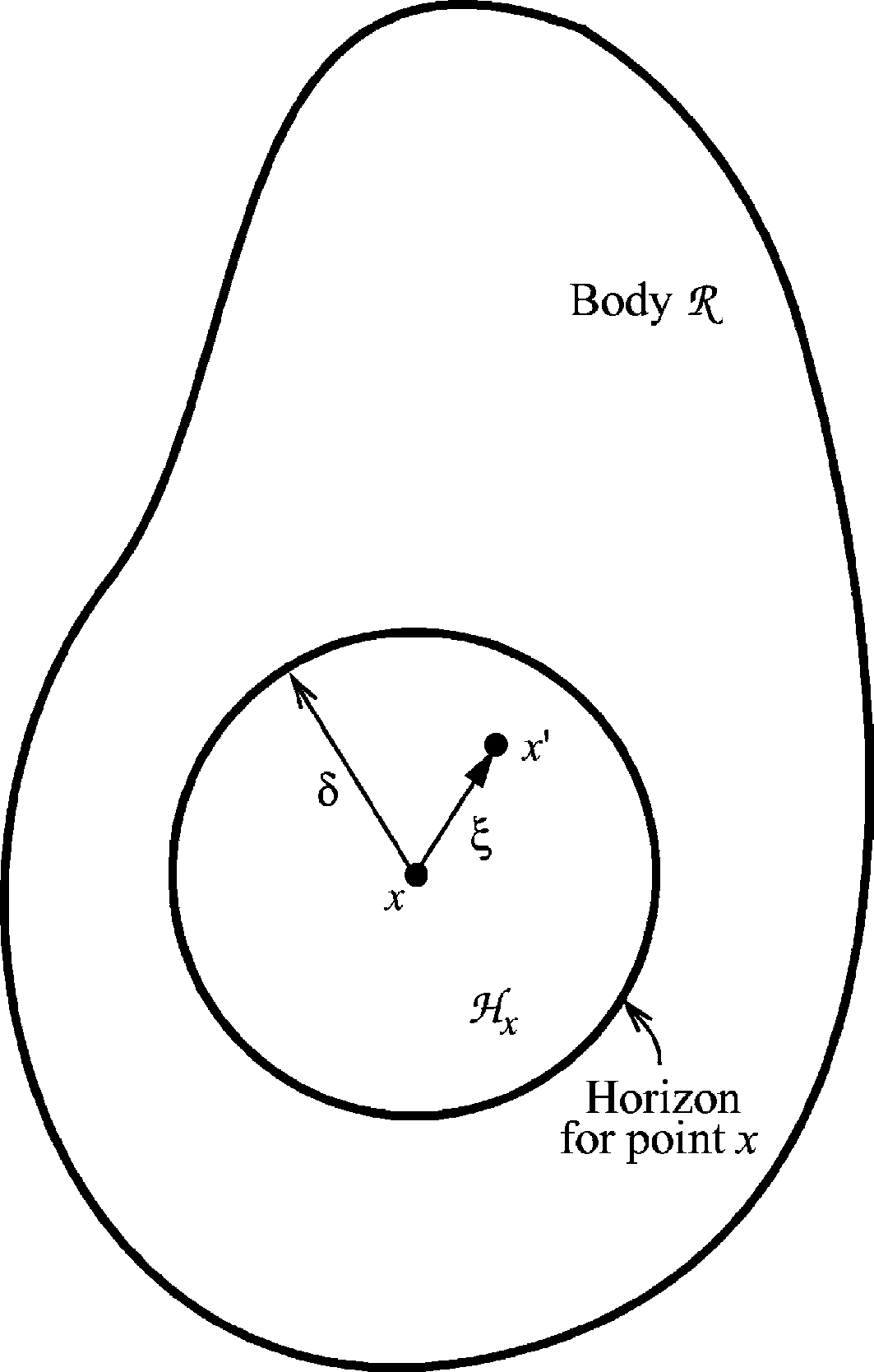
Neighborhood
\[ \rho \left(\mathbf{X} \right) \ddot{\mathbf{u}} \left( \mathbf{X}, t \right) = \mathbf{b} \left(\mathbf{X}, t \right) + \int_{\color{red}{H}} \mathbf{f} \left(\mathbf{\eta}, \mathbf{\xi} \right) dV \]
\(H\) assumes spherical region
whose radius = \(\delta\) (Horizon)
for convinience
Inertia & body force
\[ \color{red}{\rho \left(\mathbf{X} \right) \ddot{\mathbf{u}} \left( \mathbf{X}, t \right)} = \color{red}{\mathbf{b}} \left(\mathbf{X}, t \right) + \int_H \mathbf{f} \left(\mathbf{\eta}, \mathbf{\xi} \right) dV \]
\(\rho \ddot{\mathbf{u}}\):Inertia force
\(\mathbf{b}\):body force per volume
Pairwise force function
\[ \rho \left(\mathbf{X} \right) \ddot{\mathbf{u}} \left( \mathbf{X}, t \right) = \mathbf{b} \left(\mathbf{X}, t \right) + \int_H \color{red}{\mathbf{f}} \left(\mathbf{\eta}, \mathbf{\xi} \right) dV \]
Evaluate how the two points interact with each other
Remember: \(\mathbf{\xi} = \mathbf{x}' - \mathbf{x}, \mathbf{\eta} = \mathbf{u}' - \mathbf{u}\)
Bond
Bond: the interaction model
e.g. Bond "Spring" to simulate elastic body
Pairwise force function \(f\) specifies
the numerical model of the bond
e.g. for Bond "Spring" : \( \mathbf{f} = C \frac{\left| \mathbf{\xi} + \mathbf{\eta} \right| - \left| \mathbf{\xi} \right|}{\left| \mathbf{\xi} \right|} \frac{\mathbf{\xi} + \mathbf{\eta}}{\left| \mathbf{\xi} + \mathbf{\eta} \right|} \)
Required properties of \(f\)
Conservation of momentum
- Linear
- \[ \mathbf{f} \left(-\mathbf{\eta}, -\mathbf{\xi} \right) = -\mathbf{f} \left(\mathbf{\eta}, \mathbf{\xi} \right) \]
- Angular
- \[ \left(\mathbf{\xi} + \mathbf{\eta} \right) \times \mathbf{f} \left(\mathbf{\eta}, \mathbf{\xi} \right) = \mathbf{0} \]
∴ Force along current relative pos.
Elastic body
Depends only on distanece \(y = \left|\mathbf{\xi} + \mathbf{\eta} \right|\)
The microelastic material: \[\mathbf{f} \left(\mathbf{\eta}, \mathbf{\xi} \right) = \frac{\mathbf{\xi} + \mathbf{\eta}}{\left| \mathbf{\xi} + \mathbf{\eta} \right|} f \]
\[f = \frac{\partial w}{\partial y} \left(y, \mathbf{\xi} \right) \]
\(w\) is microptential
Isotropic elastic body
\[f = cs\]
- \(c\): constant, similar to spring coef.
- \(s\): bond strech, equivalent to strain \[s = \frac{y - \left| \mathbf{\xi} \right|}{\left| \mathbf{\xi} \right|} \]
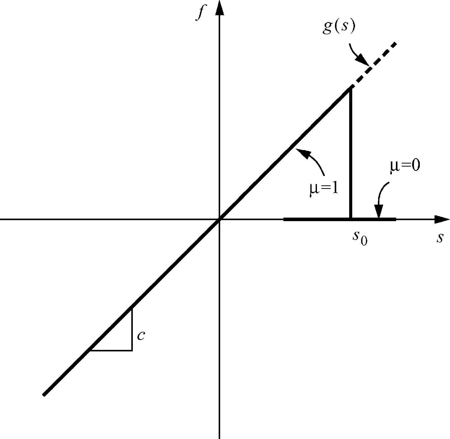
Failure
Protytype Microelastic Brittle model: \[f = cs \cdot \mu \]
\(\mu\): the bonds exists or not
- \(0\), if \((s > s_0)\) = failure has never happend
- \(1\), otherwise
\(s_0\): "critical streth"
material constant for failure criterion
How does PMB work?
| A-A' | 13 bonds | 13 bonds | 13 bonds |
|---|---|---|---|
| B-B' | 13 bonds | 11 bonds | 8 bonds |
| state | Isotropic | Anisotropic | Failure |
Damage function
\[\phi \left( \mathbf{X} \right) = \frac{\int_H \mu \left(\mathbf{X}\right) dV}{\int_H dV} \]
| Num. of bonds(\(\mu\)) | All | less | nothing |
|---|---|---|---|
| \(\phi\) | 0 | 0<1 | 1 |
| damage | Never | some | complete |
Model params of PMB
- spling-like constant: \(c\)
- \[c = \frac{18k}{\pi \delta^4}\]
- critical strech: \(s_0\)
- \[s_0 = \sqrt{\frac{5 G_0}{9 k \delta}} \]
- \(k\): bulk moduls
- \(G_0\): The work required to break all bonds per unit area
Improvements
Models mentioned above is very basic, sightly too simple
Many improved models were proposed before and after this paper
Check them before you apply
Numerical method for Peridynamics
Contents
- Introduction
- Prehistory of Peridynamics
- Peridynamics theory
- Numerical method for Peridynamics
- Result and conclusion
- My opinion
Discritized equation
| \[ \rho \left(\mathbf{X} \right) \] | \[ \ddot{\mathbf{u}} \left( \mathbf{X}, t \right) \] | \[ = \] | \[ \mathbf{b} \left(\mathbf{X}, t \right) \] | \[ \int_H \] | \[ \mathbf{f} ( \] | \[ \mathbf{\eta}, \] | \[ \mathbf{\xi} \] | \[ ) \] | \[ dV \] |
| ↓ | |||||||||
| point number \(i\), time step \(k\) | |||||||||
| \[ \rho_i \] | \[ {\ddot{\mathbf{u}}_i}^k \] | \[ = \] | \[ {\mathbf{b}_i}^k \] | \[ \sum_j \] | \[ \mathbf{f} ( \] | \[ {\mathbf{\eta}_{ij}}^k, \] | \[ \mathbf{\xi}_{ij} \] | \[ ) \] | \[ V_j \] |
Discritized PMB
\[ {\mathbf{f}_{ij}}^k = \left( c {s_{ij}}^k \cdot {\mu_{ij}}^k \right) \mathbf{n} \]
- \( {s_{ij}}^k = \frac{\left| \xi_{ij} + {\eta_{ij}}^k \right| - \left| \xi_{ij} \right|}{\left| \xi_{ij} \right|} \)
- \( {\mu_{ij}}^k = \begin{cases} 1 & \forall \kappa < k \quad {s_{ij}}^\kappa < s_0 \\ 0 & \text{otherwise} \end{cases} \)
- \( {\mathbf{n}_{ij}}^k = \frac{\xi_{ij} + {\eta_{ij}}^k }{\left| \xi_{ij} + {\eta_{ij}}^k \right|} \)
Stable condition
From 1-dim analysys:
\[ \forall i \quad \Delta t < \sqrt{\frac{2 \rho_i}{\sum_j \frac{\partial \mathbf{f}_{ij}}{\partial \mathbf{\eta}_{ij}} V_j }} \]
Depends on \(\delta\) (\(\sum_j\)), not \(\Delta x\)
Boundary condition
| conditon | fixed value |
|---|---|
| force | \(\mathbf{b}\) |
| displacement | \(\mathbf{u}\) |
Points arrengement
- Arrange points along the body shape
- Calculate volume for a point, use
- Delaunay triangulation
- Voronoi diagram

Simply put, no meshing
Result and conclusion
Contents
- Introduction
- Prehistory of Peridynamics
- Peridynamics theory
- Numerical method for Peridynamics
- Result and conclusion
- My opinion
Condition of growing crack
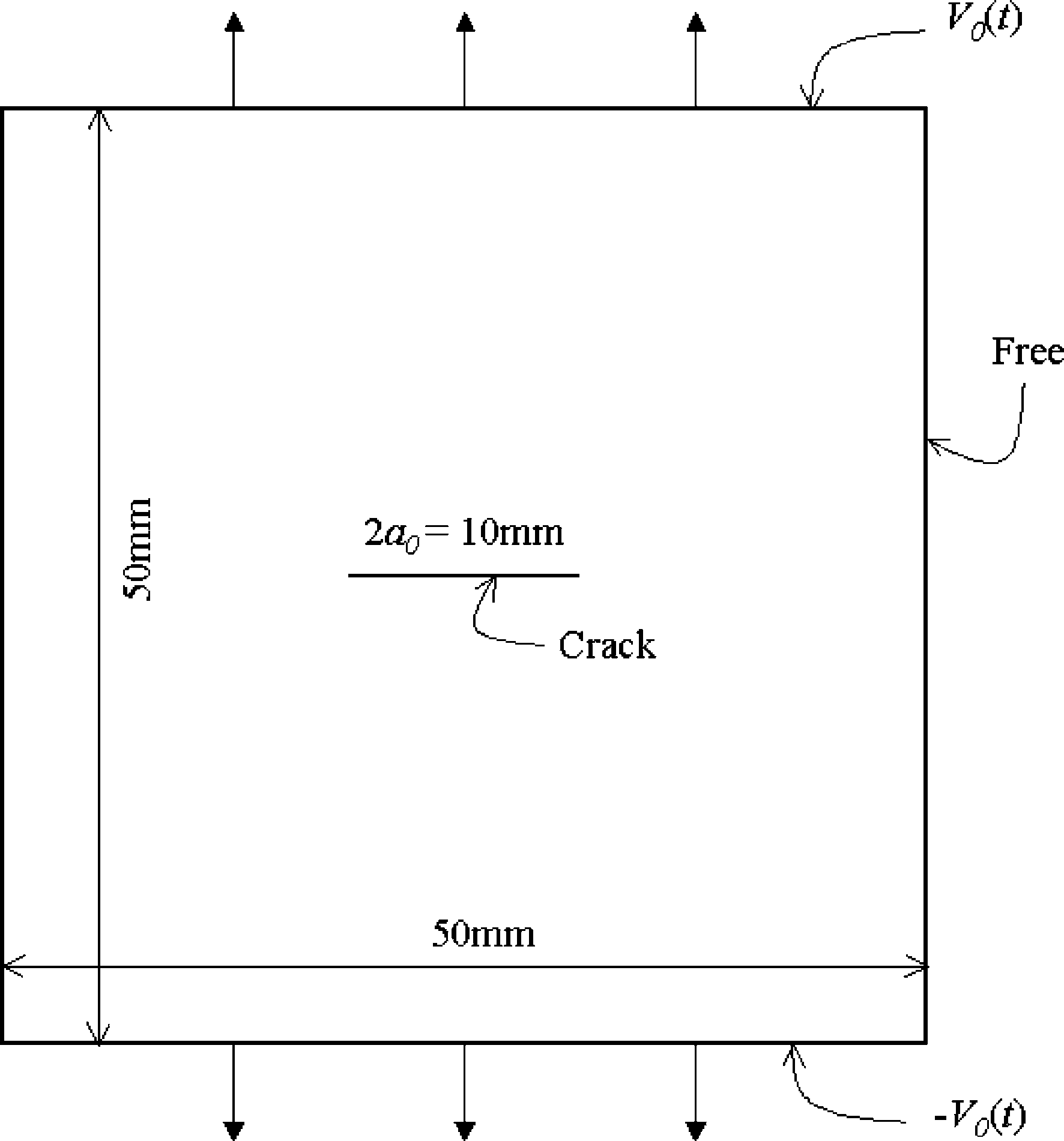
- \(\rho = 8000 \)[kg/m3]
- \(E = 192 \)[GPa]
- \(s_0 = 0.02 \)
- \(\delta = 1.6 \)[mm]
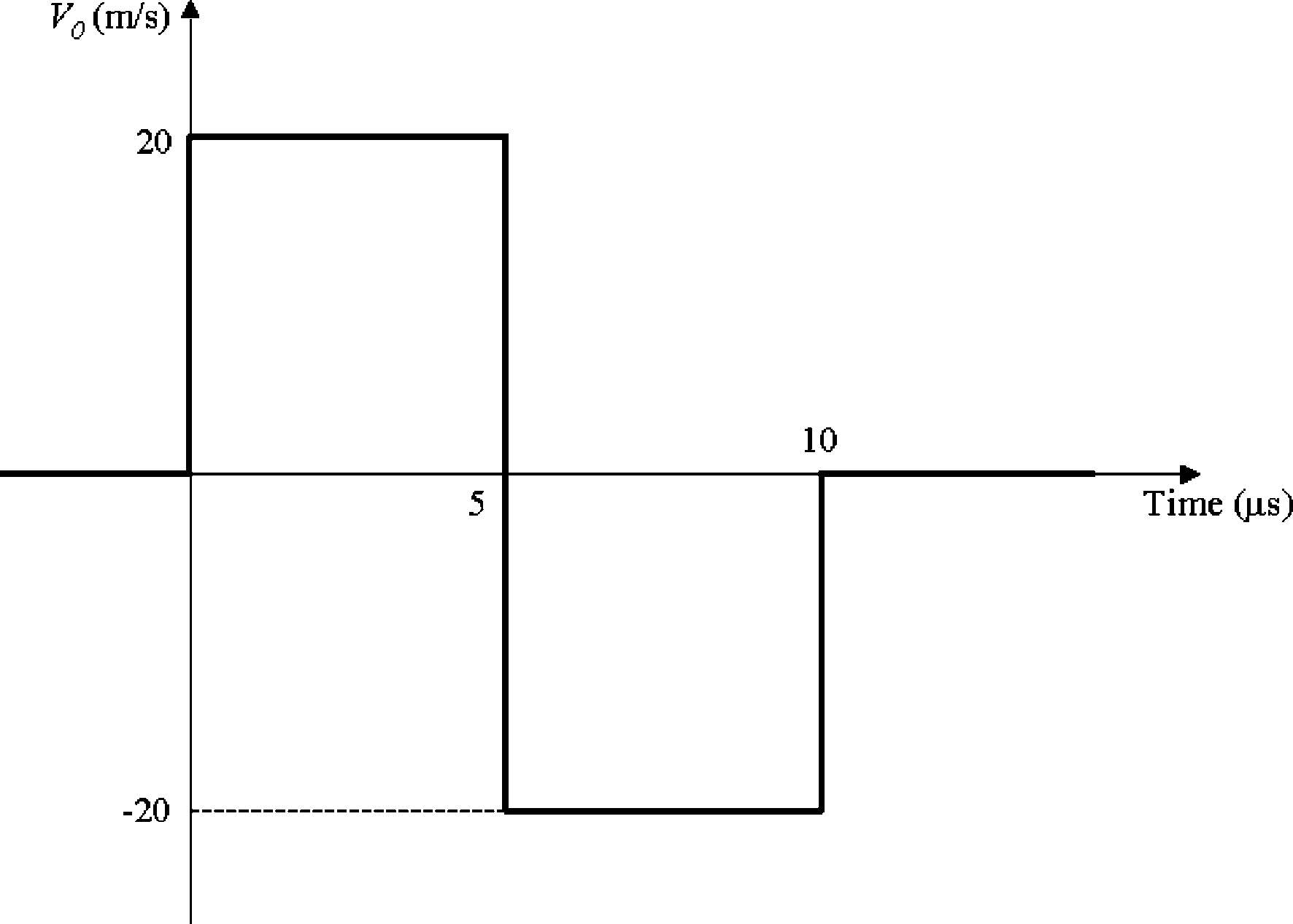
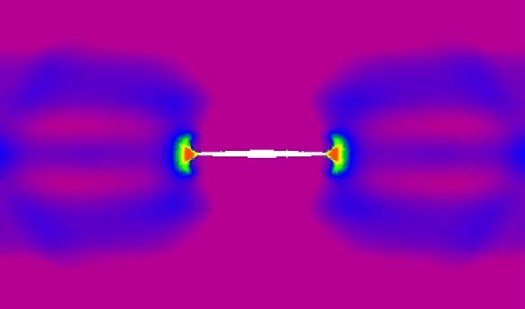
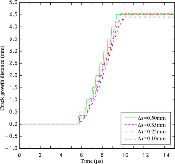
Result of growing crack
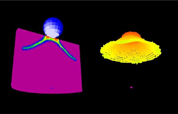
Ball impacts on cylinder
Material: glass
- \(\rho = 2200 \)[kg/m3]
- \(k = 14.9 \)[GPa]
- \(s_0 = 0.0005 \)
- \(\Delta x = 0.5 \)[mm]
- \(\delta = 1.5 \)[mm]
Result of cylinder
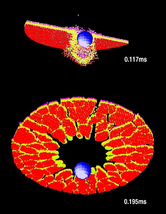
Ball impacts on plate
Same material (glass)
Result of plate
Conclusion
- New physical theory Peridynamics is for Solid Mechanics
- This paper proposed numerical method for Peridynamics
- The method is meshfree and good at simulate cracks and failure
- Failure of glass was computed and the result were shown
- This paper is the first and original numerical method for Peridynamics, so current research should be improve this method
New numerical method based on Peridynamics is expected simply to solve violent deformation and failure of solid body
Advantages than SPH
No need of spatial derivatives
- No need of neighboring search
- No tensile instability
My opinion
Contents
- Introduction
- Prehistory of Peridynamics
- Peridynamics theory
- Numerical method for Peridynamics
- Result and conclusion
- My opinion
My opnions for
- Is this "particle method"?
- How useful for fluid dynamics?
Is this particle method?
- Prof. Shibata (NIT, Gifu) said
- Not particle method but particle-based method
- My opinion
- Definitely "No"
- This is Lagrangian grid method
particle or grid?
- Grid Method
- Fixed connection between computing points
- Particle Method
- Changeable connection between computing point at every time steps
Eulerian or Lagrangian
- Eulerian method
- Fixed computing points on space
- Lagrangian Method
- Movable computing points
How about Peridynamics?
- Computing points move when each time
- → Lagrangian
- Bonds (connection) are set up by initial condition
- → Grid
∴ Peridynamics is grid method (Lagrangian)
Is this connected-DEM?
Discrete Element Method
= Particle method in a broad sense
Difference from DEM
| connected-DEM | Peridynamics | |
|---|---|---|
| Shape of Element | Sphare | Not specified |
| Interaction from | Collisioned | Bond |
| Force model | Kelvin-Voigt | Pairwise force function |
| Theory based on | discontinuous body | Continuum dynamics |
| Instance | exists | not exists |
Peridynamics is NOT family of DEM
Solving fluid dynamics?
Bonds are set up when initial condition
→ cannot unite by violently deformation
∴ Peridynamics can be applied to only Solid
But enough for Solid body
In Solid Dynamics;
- Failure by violently deformation, not unite
- Bonds and \(\mu\) can represent failue well
Fluid-Structure Interaction
Peridynamics = Lagrangian
∴ seems good with Particle method
return 0;